
Merchant Marine College, Shanghai Maritime University, Shanghai 201306, China.
*Corresponding author : Zhihui Li
Merchant Marine College, Shanghai Maritime University, Shanghai 201306, China.
Tel: 8618817502960; Email: 202230110114@stu.shmtu.edu.cn
Received: Oct 05, 2024
Accepted: Nov 15, 2024
Published Online: Nov 22, 2024
Journal: Journal of Artificial Intelligence & Robotics
Copyright: © Li Z (2024). This Article is distributed under the terms of Creative Commons Attribution 4.0 International License.
Citation: Wang H, Li Z, Wu K. A research on improving mean value engine model accuracy based on the random forest algorithm. J Artif Intell Robot. 2024; 1(2): 1013.
The indicated thermal efficiency is a core parameter that significantly affects the calculation accuracy of the fuel consumption rate in the diesel Mean Value Engine Model (MVEM). In order to improve the accuracy of the mean value engine model, a method based on Random Forest Regression Model (RF-R) was proposed to predict the indicated thermal efficiency. Using experimental universal characteristic data, the random forest regression model for predicting indicated thermal efficiency was constructed. Three-dimensional surface and contour plots of the diesel engine’s fuel consumption rate were created and the model was evaluated. The mean square errors of the training and test sets were 0.0056 and 0.0059, respectively, and the mean absolute errors were 0.0038 and 0.0043, respectively. The mean value engine model using random forest to predict the indicated thermal efficiency is simulated and verified according to the load characteristics, the results show that the mean value engine model using random forest indication thermal efficiency regression prediction has high simulation accuracy across the entire operating range of diesel engine, and compared with the model using MAP diagram calculation method, the simulation results of fuel consumption rate under each working condition are closer to the measured value, and the simulation error is less than 5%.
Keywords: Universal characteristic; Indicted thermal efficiency; Random forest regression; Simulation accuracy.
The mean value engine model, a simple model capable of describing diesel engine operating characteristics, is widely used in simulating diesel engine performance prediction and fault diagnosis. Therefore, further improving the simulation accuracy of the model has significant theoretical and engineering value. Many scholars have researched enhancing the simulation accuracy of the mean value engine model, primarily through optimizing modeling and improving core parameter prediction accuracy. Based on the Matlab/Simulink, Zhou Dong, Su Tiexiong, and others [1] considered the heat transfer in the intake system and established a diesel engine intake system model. They concluded that under steady-state conditions, simplifying the model to be adiabatic is appropriate, while under transient conditions, using an intake manifold heat exchange model improves simulation accuracy. Haitao Zhou, Ping Yan, and others [2] used a quasi-dimensional combustion model to establish a neural network model for predicting the indicated thermal efficiency of a common rail diesel engine based on five variables: speed, injection timing, excess air coefficient, injection duration, and injection pressure. This approach addressed the lack of suitable virtual prototypes and the low accuracy of the mean value engine model in electronic control system development. Chuanlei Yang, Wenle Zhang, and others [3] employed GT-power software to build a one-dimensional steady-state diesel engine mean value simulation model. They proposed a dual response surface fitting method to solve the problem of handling turbocharger characteristic parameters. Haiyan Wang, Yihuai Hu, and others [4] proposed a state space model with four variables for turbocharged diesel engines, ensuring real-time simulation accuracy while simplifying the sub-models, thereby laying the foundation for improving the overall model accuracy. Yuanyuan Tang and others [5], through an analysis of the airflow path in diesel engines, suggested adding a cylinder block sub-model between the scavenging manifold and cylinder sub-models. Based on AVL BOOST software, they established a two-stroke ultra-long stroke marine diesel engine model. Simulation analysis revealed that after adding the cylinder block sub-model, the simulation accuracy of various performance parameters of the diesel engine improved significantly. Notable improvements were seen in exhaust manifold temperature, scavenging manifold temperature, and main engine power simulation accuracy. Yanwu Ge, Ying Huang, and others [6] proposed a closed-loop correction method for the torque estimation of a turbocharged diesel engine mean value model based on engine speed using a Kalman Filter (KF) on the Matlab/Simulink. After correction with the KF, the steady-state simulation error of the model was reduced, and the dynamic simulation accuracy was improved to 90%.
Choosing a complex intake system model provides more comprehensive simulation results, but it increases the difficulty of model parameter calibration. Using a neural network to establish a predictive model for indicated thermal efficiency with five variables yields high prediction accuracy. However, the network structure greatly influences the model’s accuracy, its robustness is difficult to ensure, and the interpretability of the neural network’s internal mechanisms is weak. Establishing a one-dimensional mean value engine model enhances accuracy but also increases computational complexity. Utilizing a dual response surface to handle turbocharger parameters simplifies the model processing and improves simulation accuracy, but the model simplification can lead to reduced accuracy. Adding a cylinder block sub-model improves model accuracy and applicability, but it increases model complexity, requiring more computational resources and time. Applying a Kalman Filter for closed-loop correction of torque estimation provides more accurate torque estimates and real-time updates. However, it demanded a high level of model completeness, had high computational complexity, and requires experience and tuning for selecting filter parameters.
To address overfitting and lack of transparency in neural networks for predicting indicated thermal efficiency, this paper proposes using the random forest algorithm for prediction. The random forest algorithm is a powerful ensemble learning method where the regression prediction result is the simple average of multiple learners. The decision tree nodes are determined by formulas, giving the method high prediction accuracy, strong generalization ability, high interpretability of internal computations, and excellent capability to capture nonlinear relationships. Compared to optimization modeling methods, the random forest algorithm can improve model accuracy without increasing computational complexity. Additionally, it requires fewer parameter adjustments and simplifies the adjustment process.
Using the random forest algorithm, the indicated thermal efficiency was calculated with universal characteristic data obtained from experiments [7]. A random forest regression model was established using Matlab/Simulink. First, the performance of the random forest indicated thermal efficiency prediction model was evaluated. Next, the random forest regression model was used to validate the diesel engine’s universal characteristics. Finally, the random forest indicated thermal efficiency prediction model replaced the MAP interpolation module in the original diesel engine mean value engine model for simulation verification.
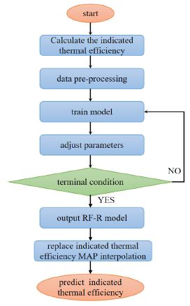
Based on the random forest algorithm [8], the indicated thermal efficiency was fitted as shown in (Figure 1). First, the indicated thermal efficiency was calculated, and the resulting data was then normalized. During model training, hyperparameters were determined based on the error. The model stopped training when the number of samples was less than the number per leaf, and no pruning was performed on the tree models within the random forest, allowing each tree to grow fully. After the model training was completed, it was saved into the mean value engine model, replacing the original indicated thermal efficiency calculation module. The inputs of this module were speed and power, and the output was the indicated thermal efficiency.
Random forest algorithm
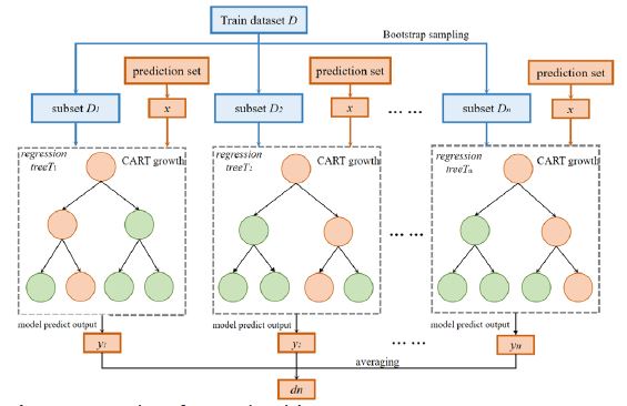
The Random Forest (RF) algorithm, proposed by Leo Breiman and other scientists, was a machine learning ensemble algorithm based on the bagging (Bootstrap Aggregating) concept [9-14]. Compared to bagging, Random Forest introduces feature randomness, significantly improving prediction accuracy without notably increasing computational load during large-scale data operations. Random Forest had a very strong learning capability, suitable for both classification and regression tasks. This paper employed a Random Forest regression model, which introduced feature randomness on top of bagging when handling regression tasks. Therefore, the Random Forest regression model had low sensitivity to outliers and missing values in the dataset and was less prone to overfitting. It was now widely used in various fields such as economics, medicine, and statistics.
The process of the Random Forest regression model [15,16] could be roughly described as follows: First, bootstrap resampling was used to extract subsets from the sample set. For a given sample set with M data points, M subsets were obtained through M resampling iterations with replacement, resulting in data subsets each containing M data points. The probability of any given data points not being selected in the sample set was.  When the sample set was sufficiently large, this could be approximated by the following formula:
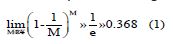
In this formula, e is the base of the natural logarithm.
According to the formula (1), the probability that a given sample did not participate in constructing a decision tree was approximately 36.8%. This meant that 36.8% of the samples in the dataset did not contribute to constructing the decision tree; this portion of the data was known as Out-of-Bag (OOB) data. OOB data could be used to test the model’s generalization performance and tuned its hyperparameters. Evaluating the model’s performance with OOB data was referred to as OOB estimation. For each decision tree, an OOB error estimation could be obtained. By summing the errors of all decision trees in the forest and then averaging them, the generalized error of the random forest (PE*) was obtained. Breiman demonstrated through experiments that OOB estimation was an unbiased estimate [17-19]. Compared to cross-validation, OOB estimation reduced the computational burden of the algorithm, improved efficiency, and produced validation results that were approximately equivalent to those of cross-validation.
The extracted M data subsets were used to train M decision trees. In the Random Forest algorithm, the default type of decision tree [20] was the CART (Classification and Regression Tree) regression tree. CART regression trees started growing from the root node, each tree grew fully without requiring pruning, and growth stopped when the tree met its termination conditions. These conditions typically included:
When the number of data points at the current node was less than a specified threshold.
When the mean squared error (MSE) at the current node was less than a predefined threshold, indicating no further split was necessary.
When the tree reached a specified depth limit.
During the growth process from root to leaf nodes, feature selection at each node was determined by calculating its mean squared error (MSE). The optimal node for splitting was selected by minimizing the MSE, as shown in the following formula:
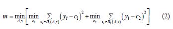
In the formula: s represents the entire training dataset at the current node. A represents the subset of features selected for the current node.
The training set was partitioned into subsets D1 and D2 based on feature A. By iterating over the values of A, the sum of the minimum mean squared errors of the output values y for subsets D1 and D2 was calculated. Eventually, by iterating through all attributes, the minimum Mean Squared Error (MSE) was determined along with the corresponding attribute and its value, providing growth information for that node. This process was repeated for each generated child node until the termination conditions were met.
After training the model, when using Random Forest for regression prediction, the final prediction result was the arithmetic average of the predicted values from each decision tree. The workflow of the Random Forest algorithm is illustrated in (Figure 2).
Construction and evaluation of the indicated thermal efficiency random forest prediction model
Calculation and preprocessing of indicated thermal efficiency: The indicated thermal efficiency of an engine could not be directly obtained from experimental data. However, the universal characteristic curve of the engine provided performance parameters such as speed, effective power, and effective fuel consumption rate. Therefore, it was necessary to extract parameters from the universal characteristic curve of the engine to calculate the indicated thermal efficiency. For a diesel engine, given the indicated power and the hourly fuel consumption, the formula for calculating the indicated thermal efficiency could be derived based on its definition, as shown in Equation (3):
In this formula: ni the indicated thermal efficiency; Pe is the effective power, obtained from the universal characteristic curve derived from experiments; Pf is the mechanical loss power, obtained from the mechanical loss model, which will be introduced in the following model; 3600 represents the energy equivalent of 1 kWh; Hu is the lower heating value of the fuel used. For ship engines, the commonly used fuel is heavy oil, and the standard lower heating value for heavy oil in China is 42,000 kJ/kg when calculating fuel consumption rate.
Moreover, the effective fuel consumption rate could be described as ge=GT/Pi
the following equation could be derived (4):
After calculating the indicated thermal efficiency, the data is normalized according to Equation (5).
Parameter selection
In the process of using the random forest regression model to predict indicated thermal efficiency, it was first necessary to determine the model parameters. In a random forest regression model, parameters that needed to be set included the minimum number of leaf nodes (minleaf) and the number of decision trees (trees). The more decision trees, the more accurate the model prediction, but the computational load significantly increased. Therefore, in this study, the Out-of-Bag (OOB) data was used for estimation. The model parameters were determined based on the OOB error estimation. The curve of OOB error estimation as a function of the number of decision trees was shown in (Figure 3). The curve of OOB error estimation as a function of the number of leaf nodes was shown in (Figure 4).
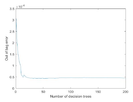
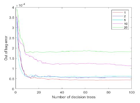
From (Figure 3), It was observed that the error decreased sharply at first and then stabilized when the number of decision trees reached 80. Therefore, to maintain computational efficiency, the number of decision trees was set to 100. From (Figure 4), it was seen that the final error was minimized when the minimum number of leaf nodes was 1. Thus, the parameter minleaf was set to 1.
RF-R evaluations and analysis
To evaluate the performance of the random forest regression algorithm for predicting indicated thermal efficiency, three metrics were selected: Root Mean Square Error (RMSE), correlation coefficient R-squared (R2), and Mean Absolute Error (MAE). RMSE and MAE were used to measure the error between the predicted values and the actual values, while R2 was used to assess the correlation between the predicted values and the actual values. The formulas were as follows.
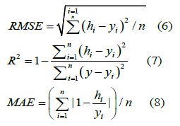
In this formula: hi is predicted thermal efficiency indicator from model output. yi is measured thermal efficiency indicator. n is the logarithm of predicted and observed values. y is the average value of observed indicated thermal efficiency.
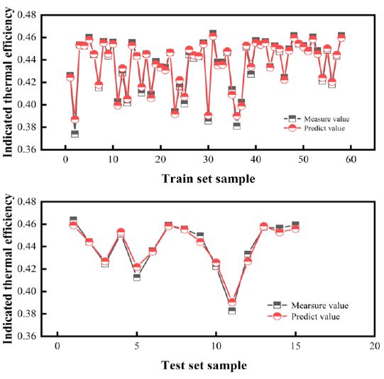
The data was divided into training and testing sets in an 8:2 ratio. Using Out-of-Bag (OOB) estimation, the model’s predicted and observed values of indicated thermal efficiency were shown in (Figure 5). Based on the evaluati on metrics, the training and testing sets exhibit mean squared errors of 0.0056 and 0.0059 respectively, mean absolute errors of 0.0038 and 0.0043 respectively, and R2 values of 0.9684 and 0.9612 respectively. These results indicated that the model demonstrated good generalization performance without overfitting. According to these assessment results, the model exhibited high predictive accuracy and strong correlation between observed and predicted values, accurately forecasting the indicated thermal efficiency of a full-load diesel engine. This performance was primarily attributed to the robust learning capability of the random forest algorithm, which effectively captured nonlinear relationships between different features.
Modules related to the mean value engine model
The mean value engine model [21-24] was a zero-dimensional mechanism model, known for its fast calculation speed and accurate external characteristic calculations. It had been widely used in the dynamic simulation of diesel engines. The mean value engine model combined the characteristics of the quasi-static model and the volume method model. Referring to the volume method model, the diesel engine was divided into several relatively independent modules. The working principle was shown in (Figure 6). The modules were linked by parameters such as pressure, flow, and temperature to form the overall diesel engine model. The mean value model simplified the in-cylinder process of the diesel engine. It treated the in-cylinder process as stable, ignoring fluctuations in temperature and pressure. The first law of thermodynamics was directly used to calculate the indicated power of the diesel engine based on indicated thermal efficiency, thereby calculating the average indicated torque [25,26].
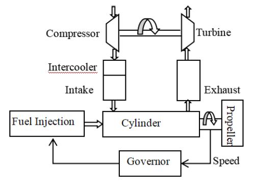
The governor adjusted the amount of circulating fuel injected into the cylinder according to the speed feedback. After the oil mist of the injection cylinder is fully mixed with the air, it exploded near the top dead center of compression, pushed the piston to do work, and converted the chemical energy of the fuel into mechanical energy with a certain thermal efficiency. The average indicated torque generated by the diesel engine could be calculated by the following formula (9):
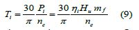
In this formula: mf is the average mass flow rate of fuel, Hu is the low calorific value of fuel, ni is the indicated thermal effi ciency, ne is the speed of diesel engine,Pi is the indicated power;
This paper only introduced the calculation method of related sub-models, and the rest can be referred to.
Indicated thermal predict model
In this article, the indicated thermal efficiency was considered as a function of rotational speed and power, as shown in formula (10):
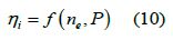
The trained random forest regression model was encapsulated in the module, and the indicated thermal efficiency MAP calculation module was replaced. The indicated thermal efficiency was predicted according to the input speed and power, and output to the next sub-module. The indicated thermal efficiency was no longer calculated by the MAP interpolation of excess air coefficient and speed, but by inputting speed and power, which was predicted by random forest regression.
Mechanical loss model
The heat loss power during the diesel engine cycle could not be ignored. Mechanical loss was considered the primary loss power of the diesel engine and was crucial for calculating its indicated thermal efficiency. However, the mechanical loss power could not be obtained by direct measurement. Therefore, this paper obtained it through the mechanical loss torque calculation sub-model in the diesel engine mean value model. The research object of this paper was a four-stroke turbocharged diesel engine, and its mechanical loss pressure could be expressed as:
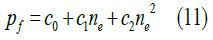
In this formula: Pf is mechanical loss pressure; ne is engine speed; C1, C2, C3 is parameter related to the specific diesel engine;
The mechanical loss torque generated by the mechanical loss pressure was calculated according to the same mode of converting the in-cylinder gas force into the output torque. The calculation formula is:
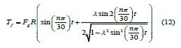
In the formula: Fg the mechanical loss pressure is the pressure on the piston according to the gas force mode; R the crank radius; λ for the crank connecting rod ratio;
The mechanical loss torque was obtained by the mechanical loss module according to formula (12), and then the mechanical loss power was obtained according to formula (13).
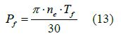
In the formula: Pf is mechanical loss power; Tf is mechanical loss torque;
The simulation model of the diesel engine in this study is built based on a turbocharged diesel engine. The main technical parameters are shown in (Table 1).
Fuel consumption rate experiment verification
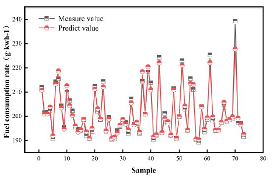
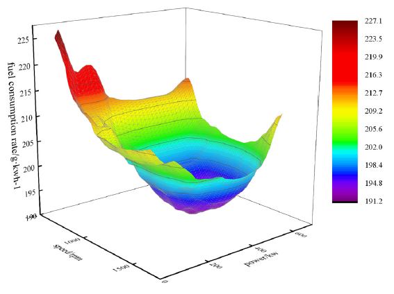
Based on the random forest regression model, the fuel consumption rate [27-30] prediction model was established.
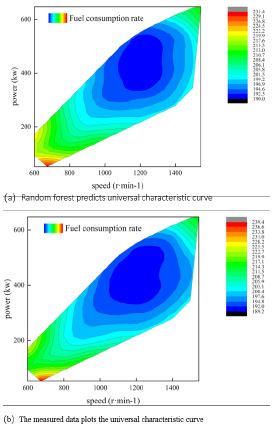
The line was shown in (Figure 7). The fuel consumption rate data across the full experiment speed and power range were predicted, and three-dimensional surface and two-dimensional contour diagrams of the fuel consumption rate were drawn. (Figure 8) showed the three-dimensional surface diagram of the universal characteristics, and (Figure 9) showed the two-dimensional contour comparison diagram of the universal characteristics. The (Figures 7,8,9) showed that the universal characteristics predicted by the random forest closely matched the measured universal characteristics curve.
Simulation model verification
The trained random forest prediction model of indicated thermal efficiency was implemented in the
Matlab function module of Matlab/Simulink, replacing the original data interpolation calculation module. Based on the load characteristics, fuel consumption rate data under different working conditions were selected for comparison of simulation results. To test the performance of the random forest algorithm across the full operating range, simulation tests were conducted at operating loads of 800 rpm, 1000 rpm, 1200 rpm, 1400 rpm, and 1500 rpm. The simulation results were shown in (Figure 10). In the (Figure 10), the error between the simulated and the measured value of the fuel consumption rate under different working conditions was compared. Method 1 used the MAP diagram to calculate the MVEM fuel consumption rate simulation result of the indicated thermal efficiency, while Method 2 used the random forest algorithm to predict the MVEM fuel consumption rate simulation result of the indicated thermal efficiency.
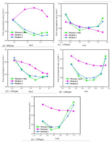
It can be seen from (Figure 10) that the fuel consumption rate calculated by the MAP diagram matched the measured rate only at low loads. At 800 rpm, it do not match the measured data at all. At 1400 rpm, the overall trend of the fuel consumption rate calculated by the MAP diagram is roughly the same as the measured value. However, the sensitivity to changes in the fuel consumption rate is insufficient, leading to a relatively large error.
In this paper, according to the universal characteristic data of diesel engine, the random forest prediction model of indicated thermal efficiency of diesel engine is successfully constructed. The model is embedded into the mean value engine model of real-time simulation, and the following conclusions are drawn:
1) The R² values of the training set and test set of the random forest indicated thermal efficiency prediction model are 0.9684 and 0.9612, respectively, indicating excellent fitting and strong correlation. In the low-speed and low-load area, the simulation error of the MVEM fuel consumption rate using the MAP diagram is slightly higher than 5%, reaching a maximum of 5.96%. The simulation error of the MVEM fuel consumption rate using the random forest algorithm to predict the indicated thermal efficiency is almost less than 5%, with a maximum of -1.45%. The remaining simulation values are closer to the measured values, indicating that the overall performance of the random forest algorithm is good. This demonstrates that using the random forest algorithm to improve the simulation accuracy of the model is feasible.
The prediction accuracy of fuel consumption rates at different loads and speeds using the MVEM calculated by the random forest is nearly higher than that using the MAP diagram. This method has the advantage of improving high prediction accuracy across the full load range.