Article Type: Research Article, Volume 2, Issue 2

Machine learning identifies crucial timeframe to reduce divorce risk

Pan Soonsawad^1*; Phakin Wongveerapaiboon²; Suwannee Adsavakulchai²; R Holland Cheng³

¹Department of Anatomy, Mahidol University, Thailand.
²School of Engineering, University of The Thai Chamber of Commerce, Thailand.
³Department of Molecular and Cellular Biology, University of California, USA.

*Corresponding author: Pan Soonsawad,
Department of Anatomy, Mahidol University, Bangkok, 10400, Thailand.

Email: pan.soo@mahidol.ac.th
Received: Aug 30, 2025
Accepted: Oct 03, 2025
Published Online: Oct 10, 2025
Journal: Journal of Artificial Intelligence & Robotics

Copyright: © Soonsawad P (2025). This Article is distributed under the terms of Creative Commons Attribution 4.0 International License.

Citation: Soonsawad P, Wongveerapaiboon P, Adsavakulchai S, Cheng RH. Machine learning identifies crucial timeframe to reduce divorce risk. J Artif Intell Robot. 2025; 2(2): 1027.

Abstract

This study aims to predict divorce risk using machine learning. Questionnaires were employed to identify key factors influencing divorce decisions, categorized into health history, childhood history, marriage history, child information, and child well-being. Three algorithms were tested: Random Forest (RF), Gaussian Naïve Bayes (GNB), and Support Vector Machine (SVM). As a result, RF was selected to predict divorce likelihood due to its superior Gini Importance value. The analysis revealed that divorces often occur within the first five years of encountering conflicts. Financial problems and infidelity consistently emerged as the leading causes. Additionally, it was found that individuals not legally registered for marriage tended to endure difficulties for a longer period, with divorce reasons being primarily minor issues.

Addressing these issues early can reduce divorce risk, strengthen relationships, enhance family stability, and contribute to societal well-being, and can also be applied to other social challenges.

Introduction

Since the 1970s, the divorce rate has been increasing globally [1], and divorce has become a common and socially acceptable form of terminating a nuptial relationship. However, the consequences of divorce are impactful, especially for children of divorced parents who are inevitably affected adversely [2]. The children might be faced with the decision of residing with either one of their parents or a relative, and this circumstance can result in psychological implications and increase the likelihood of developing mental health conditions, such as mood and behavioral disorders [3,4]. Across Asia, divorce rates have been on the rise, reflecting shifts in traditional gender roles, where women have historically been more dependent on men [5], Thailand mirrors this trend, with its divorce rate steadily increasing since 2004 [6]. This pattern persists even as fewer people choose to marry, underscoring broader regional changes in societal norms and relationship structures.

Machine learning was selected for its ability to address complex social issues, such as criminal relationships [7], by uncovering hidden patterns. It is used to better understand marriage dynamics, uncover key reasons for divorce, and suggest practical solutions. Studies, those by Gottman et al. [8], have utilized machine learning in divorce prediction, particularly through frameworks like the Gottman couples’ therapy model. Their longitudinal research, The Timing of Divorce [9], identifies that most divorces occur within the first seven years of marriage.

However, this study extends its approach by focusing specifically on the first five years after marital problems arise, a critical decision-making period. While Gottman’s work offers valuable predictions on outcomes, this research further enriches understanding by identifying the underlying causes of divorce, providing deeper insights for targeted interventions.

In summary, this research aims to address gaps in previous studies by using machine learning to predict not only the outcomes of divorce but also the critical decision-making period within the first five years when confronted with a conflict. This period is identified as being the most vulnerable for couples, where key risk factors—such as infidelity, and financial instability—play a decisive role in separation. By combining a focus on predictive modeling, this study seeks to provide a comprehensive tool for understanding and potentially mitigating the causes of divorce, which could be extended to address other social problems in the future.

Results

Designing and data collection

The problem of divorce in Thai Families has been increasing since 2004 [6]. The consequences of divorce impact children with psychological implications and mental health conditions, such as mood and behavioral disorders. This report focuses on individuals with divorce status who are of Thai nationality and have at least one child in the marriage. The children are aged three to eighteen years old providing a specific target population for the analysis which enhances the study’s validity. The population of mixed-status can be broken down into groups of 20 married participants, 17 divorced, 7 separated, 3 widowed, and 5 single for a total of 52 people.

Interestingly, among the married participants, females were the majority, accounting for 79% (41 participants), while males comprised the remaining 21% (11 participants). This is determined to be factual as it is the actual status of the participants instead of having a married status equaling “married” and all other statuses equaling “divorced”. Additionally, all participants were eighteen or over and had at least one child aged three to eighteen. According to the machine learning process, the experimental dataset must be transformed from text (answers from the questionnaire) to numbers 0, 1, 2, 3, 4, and 5 by their choices. These numbers do not represent scores but are simply a way to transform the text responses into a numerical format for machine learning purposes. The attribute “Divorce” is a class for labeling the data.

Representing divorce or marriage by substituting those whose status is married=0, divorced 72=1. This transformation was performed to prepare the data for machine learning analysis. The final dataset, after all substitutions, is shown in Supplementary (Table S1).

The modeling development

This study recognizes the importance of hyperparameter optimization in achieving the best performance and making an accurate comparison of their relative performance. The results are summarized in (Table 1).

In the competition to predict divorce likelihood, Random Forest (RF), Gaussian Naïve Bayes (GNB), and Support Vector Machine (SVM) emerged as the top contenders. Both RF and SVM achieved an accuracy of 93.75%, outperforming other models in minimizing errors, while GNB lagged at 81.25%. GNB was ulultimately eliminated due to lower performance in accuracy, F1-Score, and precision, along with the highest Root Mean Squared Error (RMSE) at 43.30%. In addition, RF and SVM demonstrated a more balanced F1-Score (0.94), indicating better equilibrium between correctly identifying divorced individuals (high recall) and minimizing false positives (lower specificity) compared to GNB. However, all models exhibited a bias towards the divorced class.

Evaluation

To evaluate the models’ performance, SVM achieved the same accuracy as RF but showed a lower cross-validation score, with RF scoring 80% and SVM scoring 75.28%, as shown in (Table 1).

Accordingly, the Random Forest algorithm was chosen to determine the likelihood of divorce due to its additional advantages. One notable feature of Random Forest is its ability to compute feature importance using the Gini Importance [10] metric. This is calculated from the feature_importances_ attribute of the sklearn ensemble. Random Forest Classifier, were the sum of all feature importance values equals 1.00. For the impurity-based Feature Importance, the higher the value the more importance the feature signifies. It can be seen that feature Q29-A01 has a Gini Importance value of 0.21, representing the highest value of 20.93 % out of all features as shown in (Table 2). Therefore, feature Q29-A01 is taken into consideration for further study of divorce data.

Additionally, The Gini algorithm is used in the calculations to select what qualifies as the classification criteria. If the Gini value is very high, this indicates that the data is mixed. If the value is zero then the data is considered all in the same group (usually found in leaf nodes). (Figure 1) shows the trend of those who are divorced when answering question 29, The duration of the problem before deciding to separate your partner with the option of the within 5 years shown as feature Q29-A01.

Deployment

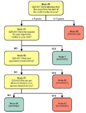
For example, the tree structure of the Random Forest algorithm has 9 nodes and has the following tree structure (Figure 1). The tree structure of the Random Forest algorithm represents the example 5-rule based as follows:

If the duration of the problem before deciding to separate is <=5 years (node #0), then the couple divorces (node #8).

If the duration of the problem before deciding to separate your couple is >5 years (node #0) and the primary cause of your arguments is related to children (node #1), then the couple remains married (node #7).

If the duration of the problem before deciding to separate your couple is >5 years (node #0), the primary cause of your arguments wasn’t related to children (node #1), and the frequency arguments about nothing (node #2), then the couple divorces (node #6).

If the duration of the problem before deciding to separate your couple is >5 years (node #0), the primary cause of your arguments wasn’t related to children (node #1), the frequency arguments about something else (node #2), and get divorced because a spouse cheating (node #3), then the couple divorces (node #5).

If the duration of the problem before deciding to separate your couple is >5 years (node #0), the primary cause of your arguments wasn’t related to children (node #1), the frequency arguments about something else (node #2), and didn’t get divorced because a spouse cheating (node #3), then the couple remains married (node #4).

(Table 3) shows the questionnaire is related to various aspects of personal relationships and experiences and is indicative of predicting or understanding divorce-related analysis and outcomes. Out of sixty questions in the online questionnaire, only twelve questions with forty-two features were related to the likelihood of divorce, with a brief interpretation of each question as follows:

Group A: The question group with the most significant impact on the decision to divorce focuses on the period when couples first began encountering issues in their relationship, which eventually led to divorce (Question 29). This question focuses on the time it took for individuals, to indicate the level of tolerance and efforts for conflict resolution. The reasons for divorce play a crucial role in influencing this decision-making process (Question 30). This question explores the reasons for the decision to separate, shedding light on the key factors leading to divorce or separation.

Group B: The question group related to the duration of married life before divorce. This question seeks to understand the duration of individuals’ current relationships, providing insights into the stability and longevity of their partnerships (Question 26). Additionally, the frequent issues that couples argue and what recurring topics of conflict contributed to their decision (Question 28). This question delves into the reasons behind arguments, highlighting potential stressors or issues.

Group C: The question group related to the reasons for choosing a partner (Question 22). This question explores the motivations and criteria for choosing a life partner, providing insights into the factors of their marital decisions. The age at which the first child was born (Question 32), and the age when began to live with their couples (even if not officially married, but cohabiting in the same household) focuses on understanding the factors influencing relationship formation and the timing of significant life milestones before or during cohabitation (Question 24).

Group D: Other questions, such as those about divorce studies and family dynamics, can be important considerations. The number of previous partners (Question 25), the age of first sexual intercourse (Question 12). This question seeks to understand the age at which individuals had their first sexual experience, which can be relevant in the context of relationships and sexual history. The frequency of arguments with a partner (Question 27), reflects on communication and relationship quality. The partner’s marital history (Question 17), can potentially influence their attitudes toward relationships based on their family background. The number of children (Question 31), focuses on aspects of the relationship and personal history that may play a smaller role in the decision to divorce.

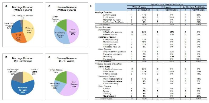
(Figure 2a-e) shows the relationship between the duration of conflicts to divorce and other questions in several dimensions, such as the duration of marriage, the reason for divorce, and the reason for frequent arguments. Among the people who divorced when they had a conflict within 5 years, 44% of marriages ended within the first 5 years, 28% lasted 5-10 years, and 24% extended beyond 10 years (Figure 2a)). Notably, 60% of individuals without a marriage certificate reported marriage durations exceeding 10 years, compared to only 4% of unregistered marriages within the 5-year range (Figure 2b).

Divorce reasons varied significantly depending on the duration of the marriage. Within the first 5 years, primary causes, including infidelity and financial issues, accounted for 46% of divorces, while secondary causes such as family interference and mental abuse contributed 38%. Minor causes, including substance abuse and incompatibility, were reported in 16% of cases (Figure 2c). In contrast, for marriages lasting 5-10 years, primary causes dominated at 60%, with secondary and minor causes contributing 20% (Figure 2d).

There is also interesting information in (Figure 2e), it presents the conflict of marriages ending in divorce across different categories. For a group conflicted to divorce within 5 years, the primary reasons for divorce were infidelity (25%) and financial issues (21%), followed by extended family problems (12%) and mental abuse (12%). Conflicts most often arose from infidelity (25%) and financial issues (18%) with secondary causes including work-related stress (11%), children (9%), and extended family disputes (4%). In the 5 to 10-year group, all individuals had been married for 5 to 10 years, possibly due to the small sample size. However, infidelity was the leading cause of divorce (40%), followed by financial issues (20%) and mental abuse (20%). Therefore, in this group, conflicts seemed to stem from minor issues. Among those without a legal marriage certificate, there is no clear reason for divorce in this group. This aligns with the frequent conflict, minor issues account for 29%, the same percentage as those who reported never arguing. Other causes, such as financial issues, work-related problems, and alcohol-related issues, each accounted for 14%.

Table 1: Results from All 3 types of Algorithms. This table presents the performance metrics of three different machine learning algorithms: Random Forest, Gaussian Naïve Bayes, and Support Vector Machine (SVM). This table is covered by the Creative Commons Attribution 4.0 International License.

Table 2: Gini importance of random forest Algorithm. This table shows which question group had the highest proportion of divorces. Question 29 had the highest proportion at 0.22, followed by Question 30 at 0.21. This table is covered by the creative commons attribution 4.0 International License.

Table 3: Grouping questions and their relationship to gini importance. This table is covered by the creative commons attribution 4.0 International License.

Discussion

The Gaussian Naïve Bayes algorithm was excluded due to lower accuracy and higher RMSE, while Random Forest outperformed Support Vector Machine (SVM) in cross-validation. Despite this, SVM demonstrated strong class-separation capabilities, making it valuable for future predictive tasks. The results reveal that the duration of marital problems plays a critical role. Our findings suggest that the first five years after encountering marital issues appear to be a crucial decision-making window. Couples who persevere through these challenges or find solutions during this period, demonstrating patience, might have a higher chance of staying together. Conversely, those contemplating divorce within this timeframe may be at a higher risk of separation. For those experiencing problems within five to ten years, the finances and infidelity of a spouse are important compared to other periods. For individuals who have never registered their marriage, divorces may stem from minor issues that can easily lead to separation, as they are not legally bound to each other.

The results clearly show that the timeframe is the most significant factor in the decision to divorce, and whether or not to divorce depends on the problems faced. Although the first five years were the most important period, not every couple divorced within this time frame; some experienced divorce later, depending on other factors. Thus, Infidelity and financial issues are identified as the primary reasons that tend to have a greater emotional impact than others, making it easier for people to react strongly when considering divorce.

Consequently, the Random Forest model’s strong performance in this study showcases the potential of machine learning to analyze relationship dynamics and identify hidden patterns. However, it’s important to emphasize that these models are tools to aid understanding, not replacements for human expertise in navigating complex social issues. Lastly, the importance of addressing ethical concerns in AI research, such as data privacy, potential biases, and algorithmic transparency [7]. Future studies should address these concerns to ensure that predictive models are implemented responsibly, safeguarding individual rights while contributing to meaningful social insights.

Methods

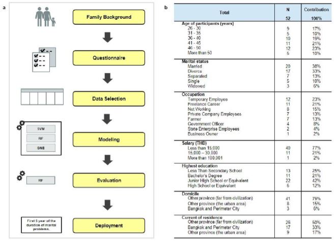
In terms of data analysis, the Cross-Industry Standard Process for Data Mining (CRISP-DM) is a widely used methodology for data analyses that consists of six main phases: Business Understanding, Data Understanding, Data Preparation, Modeling, Evaluation, and Deployment [11]. A summary of the working process is shown in (Figure 3a) as follows:

Business understanding

The traditional Thai belief in monogamy regards marriage as a lifelong commitment that has been challenged by various factors influenced by global culture. Consequently, the trend of divorce has been increasing in Thailand, challenging the Buddhist way of valuing the sanctity of marriage as a vital aspect of Thai society.

Data understanding

The research was conducted using questionnaires that collect environmental data to determine the most significant factor to influence the decision to divorce. The questions are divided into categories such as personal information, including income and educational background, health history, childhood history, marital history, children’s well-being, and the residential environment.

All questionnaires used in this study have been validated by the author’s university to ensure compliance with internationally recognized human research ethical guidelines, including the Declaration of Helsinki Belmont Report, CIOMS Guidelines, and the International Conference on Harmonization in Good Clinical Practice This validation ensures that the study adheres to ethical standards for human research, safeguarding the rights and well-being of participants while maintaining the integrity of the research process. By following these established guidelines, the study upholds the highest standards of ethical conduct in human research (No. UTCCEC/Expedited007/2565).

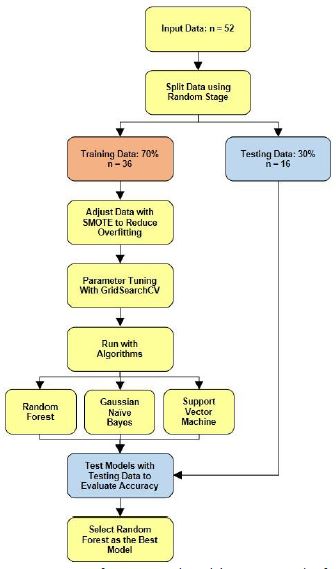
The primary source for this study is an online questionnaire. Krejcie and Morgan Tables [12] is used for sample size calculation which considers the proportion of traits of interest in the population, the desired level of tolerance, and the confidence level. The sample size of 60 surveys is relatively small, but it is adequate to conduct initial analysis and explore the relationship between predictor variables and divorce outcomes. The sample size of 52 out of a population of 60 indicates a high response rate, which is a positive aspect of the study. (Shown in part of Figure 3b).

Data preparation

Data Preparation is the process of rationalizing and transforming raw data into a form that is suitable for use in machine learning. This is a crucial step as the quality and characteristics of the data can greatly impact the accuracy and usefulness of the results, with sub-processes as follows:

Feature selection

Feature selection to predict the likelihood of divorce is set up based on several categories. Some questions that were not related to the participants’ marital life were excluded, such as personal history, health history, children’s information, etc. Until only a set of 12 questions remained that matched the prediction of divorce outcome as shown in the Supplementary Information.

Data cleaning

It was necessary to directly ask the participants to confirm relevant personal information such as marital status as well as any complex cultural aspect to ensure the accuracy of the data. By carefully cleaning and verifying the data, researchers can improve the quality and reliability of the results and enhance the validity of the study. The use of ordinal scale and nominal polytomous scale questions allows for more nuanced responses and provides more insightful data for analysis.

Data transformation

All questions and answers are converted to numeric code to enable machine learning algorithms to understand and analyze the format. For example, question 12 which asks, “How old were you when you had your first sexual intercourse?” is converted to Q12. The question has the following available responses: Never had sex, under 20 years old, 20-25 years old, 26-30 years old, and 31 years old and over, and these are converted to 1, 2, 3, 4, 5 accordingly. Furthermore, some data points that might bias the model’s classification were modified or removed. For example, answers stating Never divorced were excluded from the features. Furthermore, certain data items were combined to facilitate processing. For instance, responses indicating less than 1 year and between 1-5 years for questions 26 and 29 were grouped.

Transforming questions with multiple answers into attributes is a technique in machine learning. This process is called one-hot encoding and involves creating a new binary attribute. For example, question 22 asks “What were the reasons for deciding to choose a spouse?” and the answers are Appearance, Love, Financial, Character, and Family approval. These will be transformed into attributes Q22-A1, Q22-A2, Q22-A3, Q22-A4, and Q22-A5. For any positive selection by the participants, the value will be substituted for 1 as an input and 0 for all others when not selected.

As a result, all 42 features have a string of values that is ready for analysis. Each row represents one participant response representing a married couple. The columns represent questions in order of attributes Q12, Q17, Q22-A1, Q22-A2, Q22-A3, Q22-A4, Q22-A5, Q24, Q25, Q26-A01, Q26-A02, Q26-A03, Q27, Q28-A01, Q28-A02, Q28-A03, Q28-A04, Q28-A05, Q28-A06, Q28-A07, Q28-A08, Q28-A09, Q28-A10, Q28-A11, Q28-A12, Q28-A13, Q29-A01, Q29-A02, Q29-A03, Q30-A01, Q30-A02, Q30-A03, Q30-A04, Q30-A05, Q30-A06, Q30-A07, Q30-A08, Q30-A09, Q30-A10, Q31, Q32, and Divorce.

Modeling

Three machine learning algorithms, namely Random Forest, Gaussian Naïve Bayes, and Support Vector Machine were utilized to analyze the collected data. In the first algorithm, Random Forest [18] each tree is trained on a bootstrapped sample of the training data and a random subset of the features. The trees are then combined through a majority vote or by averaging their predictions. The process uses the Python scikit-learn library sklearn. ensemble. Random Forest Classifier [16], which subsequently utilizes the CART (Classification and Regression Trees) algorithm very similar to C4.5, but it differs in that it supports numerical target variables (regression) and does not compute rule sets. CART constructs binary trees using the feature and threshold that yield the largest information gain at each node [17].

Furthermore, the second algorithm, Gaussian Naïve Bayes classifier [22] uses the Python scikit-learn library sklearn .naive_bayes. Gaussian NB [18]. The last algorithm is Support Vector Machines (SVMs) [24]. This research uses the Python scikit-learn library sklearn. svm. SVC [19] by calling to set the kernel type using the linear 〈x, x′〉 method.

This study employed GridSearchCV [20] for hyperparameter optimization, using accuracy as the key metric for model selection via 5-fold cross-validation. Different machine learning models were investigated:

The Random Forest model focused on the number of decision trees (1,000, 2,000, or 3,000), the maximum depth of each tree (4, 8, or 16 levels), the minimum number of data points required to split a node (2, 5, or 10), and the minimum number of data points allowed in a final decision (leaf) of the tree (1, 2, or 4). The Gini impurity and entropy criteria were evaluated for the splitting function. Finally, it achieved the highest accuracy of 80% when using the entropy criterion for splitting data. This coincided with specific parameter settings: a maximum tree depth of 4, a minimum of 0 data points for splitting nodes, a minimum of 1 data point in leaves, and utilizing 2,000 decision trees.

Hyperparameter tuning for the Gaussian Naive Bayes model was achieved through which the var_smoothing parameter was evaluated across values ranging from 1 (e^0) to 1e-7 or 1 (e^0) to 1e-8 or 1 (e^0) to 1e-9. The Gaussian Naive Bayes model excelled with a superior accuracy of 75.28%, obtained through a variance smoothing parameter of 1 (e^0) to 1e-9.

The last one, the Support Vector Machine (SVM) classifier investigation encompassed various kernel functions (linear, radial basis function (RBF), polynomial, sigmoid), the regularization parameter (C) as (0.01, 0.1, 1, 10, or 100), gamma as (auto, 0.1, 1, or 10), and the inclusion of probability estimates (True or False). The tuning showed that the classifier delivered the best accuracy of 75.28%. The optimal configuration likely included a linear kernel with a regularization parameter (C) of 1, using gamma at 0.1, and probability estimates enabled and used RBF kernels to employ in SVM applications.

Following hyperparameter optimization via GridSearchCV, the three machine learning models were trained on the preprocessed data to predict the likelihood of divorce.

Evaluation

To evaluate the performance of the models, this study considers the following metrics: Cross-validation score, Accuracy, Root Mean Squared Error (RMSE), Precision, Recall, and F1-Score. These metrics provide a comprehensive evaluation of model performance.

Deployment

Deployment is the final stage in the machine learning process where a trained model is integrated into a real-world application.

Declarations

Data availability statement: All analytical data supporting this manuscript are provided in the Supplementary Material, (Table S1).

Author contributions statement: P.W. data Collection, preparation, analysis, writing, and visualization, S.A. conceptualization, design, and literature review, R.C. modeling, supervision, and funding acquisition, P.S. behavioral studies and problem analysis. All authors reviewed the manuscript.

Competing interests: The authors declare no competing interests.

References

1. Sadiq Fareed MM, et al. Predicting Divorce Prospect Using Ensemble Learning: Support Vector Machine, Linear Model, and Neural Network. Comput Intell Neurosci. 2022: 1–15.
2. Mira Spremo. Children and Divorce. Psychiatria Danubina. 2020: 353–359.
3. Çaksen H. The effects of parental divorce on children. Psychiatriki. 2021. https://doi.org/10.22365/jpsych.2021.040.
4. O’Hara KL, Sandler IN, Wolchik SA, Tein JY, Rhodes CA. Parenting time, parenting quality, interparental conflict, and mental health problems of children in high-conflict divorce. Journal of Family Psychology. 2019; 33: 690–703.
5. Iida A. How Do Traditional Gender Roles Influence Women’s Lives in Taiwan? An Investigation of
6. Highly Educated Women’s Willingness to Create Families. East Asia. 2022. https://doi.org/10.1007/s12140-022-09392-3.
7. Thai National Statistical. Statistical report on the number of divorce registrations. https://stat.bora.dopa.go.th/stat/marry/new/stat-gen/static.php?divorce.
8. Perc M, Ozer M, Hojnik J. Social and juristic challenges of artificial intelligence. Palgrave Commun. 2019; 5: 61.
9. Yöntem M, Adem K, Ilhan T, Kılıçarslan S. Divorce Prediction Using Correlation Based Feature Selection and Artificial Neural Networks. 2019.
10. Gottman JM, Levenson RW. The Timing of Divorce: Predicting When a Couple Will Divorce Over a 14-Year Period. Journal of Marriage and Family. 2000; 62: 737–745.
11. Breiman L. Random Forests. Mach Learn. 2001; 45: 5–32.
12. Olson D, Shi Y. Introduction to Business Data Mining. McGraw-Hill College, Columbus, OH. 2005.
13. Krejcie RV, Morgan DW. Determining Sample Size for Research Activities. Educ Psychol Meas. 1970; 30: 607–610.
14. Scikit Learn. sklearn.model_selection.train_test_split. https://scikit-learn.org/stable/modules/generated/sklearn.model_selection.train_test_split.html.
15. Chawla NV, Bowyer KW, Hall LO, Kegelmeyer WP. SMOTE: Synthetic Minority Over-sampling Technique. Journal of Artificial Intelligence Research. 2002; 16: 321–357.
16. Imbalanced-learn. imblearn.over_sampling.SMOTE. https://imbalanced-learn.org/stable/references/generated/imblearn.over_sampling.SMOTE.html.
17. Scikit Learn. sklearn.ensemble.RandomForestClassifier. https://scikit-learn.org/stable/modules/generated/sklearn.ensemble.RandomForestClassifier.html.
18. Breiman L, Friedman JH, Olshen RA, Stone CJ. Classification and Regression Trees. Routledge. 2017. https://doi.org/10.1201/9781315139470.
19. Scikit Learn. sklearn.naive_bayes.GaussianNB. https://scikit-learn.org/stable/modules/generated/sklearn.naive_bayes.GaussianNB.html.
20. Scikit Learn. sklearn.svm.SVC. https://scikit-learn.org/stable/modules/generated/sklearn.svm.SVC.html.
21. Scikit Learn. sklearn.model_selection.GridSearchCV. https://scikit-learn.org/stable/modules/generated/sklearn.model_selection.GridSearchCV.html.